


Photo by Ibrahim Boran on Unsplash
Analysis Report - Predicting if income exceeds 50K per year based on US Census Data with Simple Classification Techniques


Table of contents
Datasource
- Kaggle Notebook: US Adult Income Survey.
- Dataset: Us Adult income survey - dataset
Introduction
The US Adult Census dataset is a repository of 48,842 entries extracted from the 1994 US Census database. In this article we will explore the data at face value in order to understand the trends and representations of certain demographics in the corpus.
Then we will find the relationship between each column with the target value, and we will define the model to predict whether an individual made more or less than 50K in 1994.
Then we will compare the models which better suits the dataset.
Exploratory Analysis
The Dataset Dictionary
The census income dataset has 48,842 entries. Each entry contains the following information about an individual.
- age: The age of an individual. Integer greater than 0.
- workclass: A general term to represent the employment status of an individual (Private, Selfempnotinc, Selfempinc, Federalgov, Localgov, Stategov, Withoutpay, Neverworked. )
- fnlwgt: Final Weight. In other words, this is the number of people the census believes the entry represents. Integer greater than 0.
- education: The highest level of education acheived an individual. (Bachelors, Somecollege, 11th, HSgrad, Profschool, Assocacdm, Assocvoc, 9th, 7th8th, 12th, Masters, 1st4th, 10th, Doctorate, 5th6th, Preschool.)
- education-num: The highest level of education achieved in numerical form. Integer greater than 0.
- maritalstatus: The marital status of an individual. Marriedcivspouse corresponds to a civilian spouse while MarriedAFspouse is a spouse in the Armed Forces. Marriedcivspouse, Divorced, Nevermarried, Separated, Widowed, Marriedspouseabsent, MarriedAFspouse.
- occupation: The general type of occupation of an individual. (Techsupport, Craftrepair, Otherservice, Sales, Execmanagerial, Profspecialty, Handlerscleaners, Machineopinspct, Admclerical, Farmingfishing, Transportmoving, Privhouseserv, Protectiveserv, ArmedForces. )
- relationship: represents what this individual is relative to others. For example an individual could be a Husband. Each entry only has one relationship attribute and is somewhat redundant with marital status. We might not make use of this attribute at all. (Wife, Ownchild, Husband, Notinfamily, Otherrelative, Unmarried. )
- race: Descriptions of an individual's race. (White, AsianPacIslander, AmerIndianEskimo, Other, Black. )
- sex: The bilogical sex of the individual (Male, Female)
- Capital gain: Capital gains for an individual
- Capital loss: Capital loss for an individual.
- hoursperweek: the hours an individual has reported to work per week (continuous.)
- native-country: Country of origin of an individual. (UnitedStates, Cambodia, England, PuertoRico, Canada, Germany, OutlyingUS(GuamUSVIetc), India, Japan, Greece, South, China, Cuba, Iran, Honduras, Philippines, Italy, Poland, Jamaica, Vietnam, Mexico, Portugal, Ireland, France, DominicanRepublic, Laos, Ecuador, Taiwan, Haiti, Columbia, Hungary, Guatemala, Nicaragua, Scotland, Thailand, Yugoslavia, ElSalvador, Trinadad&Tobago, Peru, Hong, HolandNetherlands. )
- the label: whether or not an individual makes more than 50K annually.
The original dataset contains a distribution of
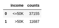
To gain insights about which features would be most helpful for this dataset, we look at the feature and the distribution of entries that are labelled >50k and <=50k.
Column : Age.
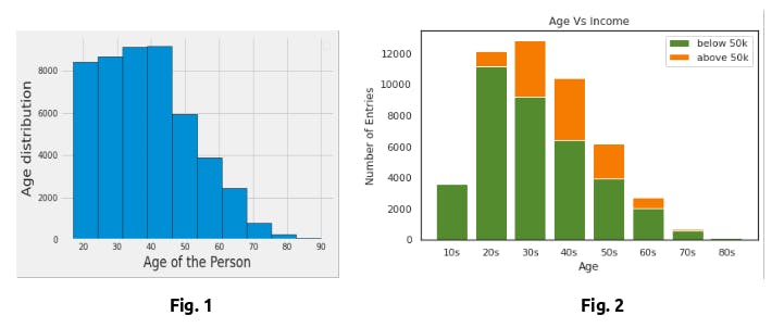
The age feature describes the age of the individual. Fig. 1 shows the age distribution among the entries in our dataset. The ages range from 17 to 90 years old with the majority of entries between the ages of 25 and 50 years. Because there are so many ages being represented, we bucket the entries into age groups with intervals of ten years to present the data more concisely as seen in Fig 2. We are considering the starting age as 14 as per dol.gov/general/topic/youthlabor/agerequire..
Looking at the graph, we can see that there is a significant amount of variance between the ratio of >50k to <=50k between the age groups. The most interesting ratios to note are those of groups 10s, 70s and 80s where there is almost no chance to have an income of greater than 50K. The ratio of entries labeled >50k to <=50k for age groups 20s, 30s, 40s and 50s vary significantly as well.
Column: Workclass
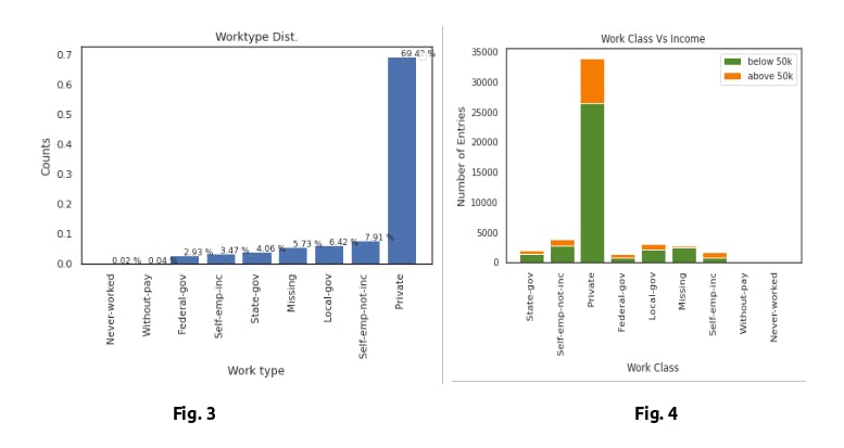
As seen in Fig. 3, the majority of the individuals work in the private sector. The one concerning statistic is the number of individuals with an Missing work class. The probabilities of making above 50K are similar among the work classes except for selfempinc and federal government. Federal government is seen as the most elite in the public sector, which most likely explains the higher chance of earning more than 50k. selfempinc implies that the individual owns their own company, which is a category with an almost infinite ceiling when it comes to earnings. The complete Work Class vs Income graph can be seen in Fig. 4. From Fig.4, we can see that individuals who work in private workclass, has more probabilities of making more than 50k.
Column: fnlgwt
Final Weight. final weight. In other words, this is the number of people the census believes the entry represents. Since this is not having any predictive power, we can remove this column.
Column: Education, Education num.
Since these two columns are representing the same data on education, we can ignore any one of them. Here to avoid more work we can ignore the categorical column
- Education: the highest level of education achieved by an individual. (Bachelors, Somecollege, 11th, HSgrad, Profschool, Assocacdm, Assocvoc, 9th, 7th8th, 12th, Masters, 1st4th, 10th, Doctorate, 5th6th, Preschool)
- educationnum: the highest level of education achieved in numerical form.
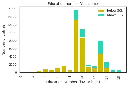
There is relationship between the highest level of education and the number of people labeled >50k and <=50k. For the most part, a higher level of education is correlated to a higher percentage of individuals with the label >50k.
Column: Maritalstatus
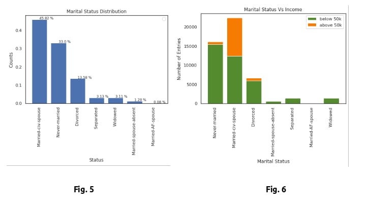
From the Fig. 6, Married-civ-spouse is having the highest probabilities of earning above 50k. Also people who never-married and divorcee, were having almost equal ratios of earning above 50k. And people who are separated, Married-AF-Spouse, Widowed were no probabilities of earning above 50k.
Column: Occupation
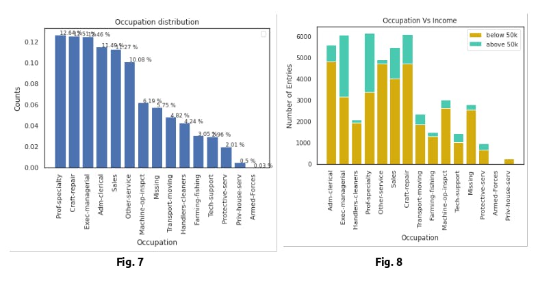
As seen in Fig. 7, there is a somewhat uniform distribution of occupations in the dataset, disregarding the absence of Armed Forces. However, looking at Fig. 8 Occupation vs Income, exec-managerial and prof-specialty stand out as having very high percentages of individuals making over 50K. In addition, the percentages for Farmingfishing, Otherservice and Handlerscleaners are significantly lower than the rest of the distribution. The one concerning statistic looking at Fig. 8 is the high number of individuals with unknown occupations.
Column: Relationship
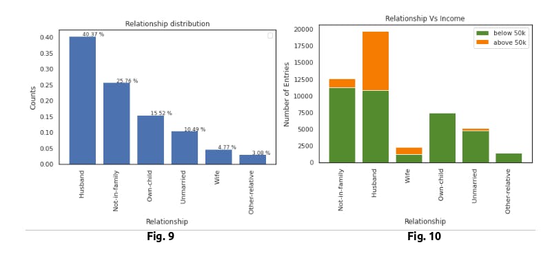
- Husbands are having higher probabilities of making over 50k
- Not-in-family and Wife were having the same probabilities of making above 50k
- Individuals who are unmarried is having lower probabilities of making above 50k
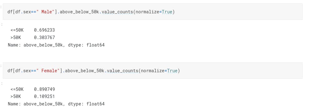
Column: Sex
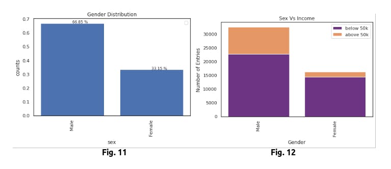
In the given dataset, there is not a normal distribution found. Percentage of male is higher than the female.
In Fig 11, we can see that there is almost double the sample size of males in comparison to females in the dataset. While this may not affect our predictions too much, the distribution of income can. As seen in Fig 12, the percentage of males who make greater than 50K is much greater than the percentage of females that make the same amount. This will certainly be a significant factor, and should be a feature considered in our prediction model.
Column: Race.
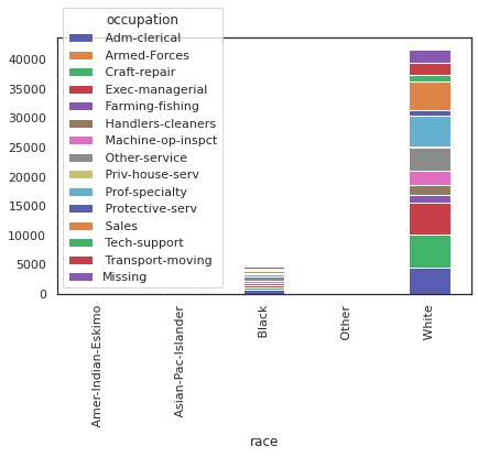
Looking at the above image, it seems like the feature could be useful in our prediction model, as Whites and Asians have a larger percentage of entries greater than 50k than the rest of the races.

However, the sample size of Whites in the dataset is disproportionately large in comparison to all other races. The second most represented group is Blacks with less than 5000 entries. The lack of equal distribution caused us to consider not utilizing this attribute in our prediction model.
Column: Capital Gain
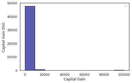
For the column, capital_gain we can see, there are many zero values. These wont have the predictive power. So we can remove this column
Column: Capital Loss
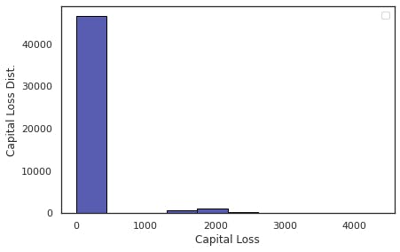
For the column, capital_loss we can see, there are many zero values. These wont have the predictive power. so we can remove this column.
Column: Hours Week
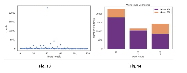
Looking at the distribution in Fig. 13 , the vast majority of individuals are working 40 hour weeks which is expected as the societal norm. Regardless of the nonuniform distribution, Fig. 14 shows that the percentage of individuals making over 50k drastically decreases when less than 40 hours per week, and increases significantly when greater than 40 hours per week.
Column: Country
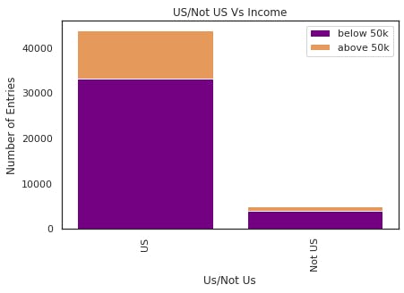
The country column is been divided into two categories US / Not Us. From the above comparison image, we can see that people is us is having a higher probabilities of making more than 50k.
Removal of Features
We also opted to not use the features: ‘fnlwgt’, ‘relationships’, and ‘capitalGains/Loss’. These features either were not useful for our analysis or had too much bad data i.e. zerovalues, unknown/private values.
Model
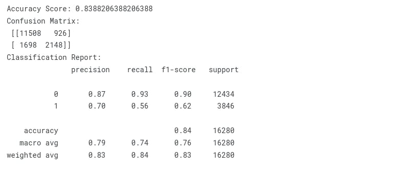
Logistic Regression
from sklearn.linear_model import LogisticRegression
lg_model = LogisticRegression()
lg_model.fit(X_train, y_train)
y_pred = lg_model.predict(X_test)
print("Accuracy Score: {}".format(accuracy_score(y_test, y_pred)))
print("Confusion Matrix:\n {}".format(confusion_matrix(y_test, y_pred)))
print("Classification Report:\n {}".format(classification_report(y_test, y_pred)))
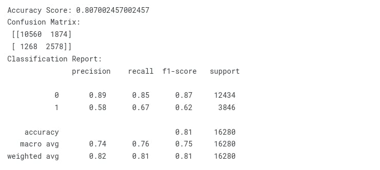
Multinomial Naive Bayes
from sklearn.naive_bayes import MultinomialNB
clf = MultinomialNB()
clf.fit(X_train, y_train)
y_pred = clf.predict(X_test)
print("Accuracy Score: {}".format(accuracy_score(y_test, y_pred)))
print("Confusion Matrix:\n {}".format(confusion_matrix(y_test, y_pred)))
print("Classification Report:\n {}".format(classification_report(y_test, y_pred)))
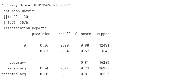
Decision Tree
from sklearn.tree import DecisionTreeClassifier
clf = DecisionTreeClassifier()
clf = clf.fit(X_train, y_train)
y_pred = clf.predict(X_test)
print("Accuracy Score: {}".format(accuracy_score(y_test, y_pred)))
print("Confusion Matrix:\n {}".format(confusion_matrix(y_test, y_pred)))
print("Classification Report:\n {}".format(classification_report(y_test, y_pred)))
Random Forest
from sklearn.ensemble import RandomForestClassifier
clf = RandomForestClassifier()
clf = clf.fit(X_train, y_train)
y_pred = clf.predict(X_test)
print("Accuracy Score: {}".format(accuracy_score(y_test, y_pred)))
print("Confusion Matrix:\n {}".format(confusion_matrix(y_test, y_pred)))
print("Classification Report:\n {}".format(classification_report(y_test, y_pred)))
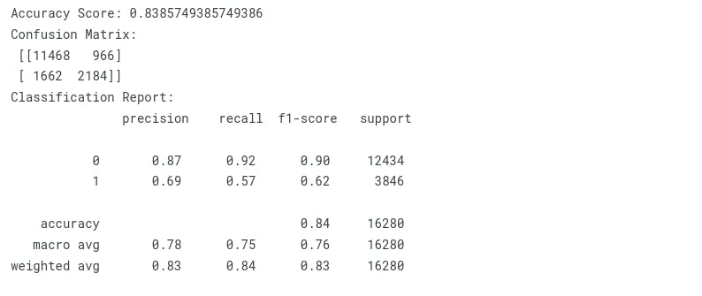
Ada Boost Classifer
from sklearn.ensemble import AdaBoostClassifier
clf = AdaBoostClassifier(random_state=40)
clf = clf.fit(X_train, y_train)
y_pred = clf.predict(X_test)
print("Accuracy Score: {}".format(accuracy_score(y_test, y_pred)))
print("Confusion Matrix:\n {}".format(confusion_matrix(y_test, y_pred)))
print("Classification Report:\n {}".format(classification_report(y_test, y_pred)))
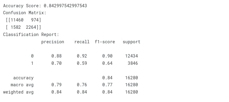
Light GBM
import lightgbm as lgb
clf = lgb.LGBMClassifier()
clf.fit(X_train, y_train)
y_pred = clf.predict(X_test)
print("Accuracy Score: {}".format(accuracy_score(y_test, y_pred)))
print("Confusion Matrix:\n {}".format(confusion_matrix(y_test, y_pred)))
print("Classification Report:\n {}".format(classification_report(y_test, y_pred)))
Model Comparison
| Algorithm | Accuracy |
| Logistic Regression | 0.8388206388206388 |
| Multinomial Naive Bayes | 0.807002457002457 |
| DecisionTreeClassifier | 0.8116707616707617 |
| ExtraTreesClassifier | 0.8182432432432433 |
| AdaBoostClassifier | 0.8385749385749386 |
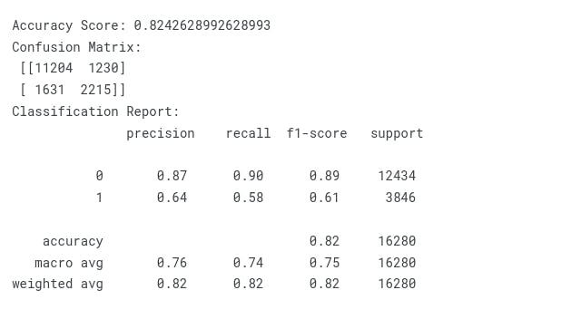
| LightGBM | 0.842997542997543 |
Inference
From the above analysis we can say that 'Light GBM ' is performing good for this dataset.